Course notes for
Section 2, Chapter 3 of the course SEG 2106
by
Gregor v. Bochmann, February 2004 (translated to English:
January 2008, revised 2009, 2010, 2011, 2012, 2013, 2015)
You know recursive equations from linear algebra. Example:
These are equations over the field of real numbers where multiplication has an inverse, the division. Therefore we can find a solution by substitution. For instance, we obtain from the first equation the following expression for x1 : x1 = 1/(1-a11) * (a21 * x2 + b1). This can be substituted into the second equation which then can be solved for x2.
The inverse operation does not exist for the union and concatenation operators that are used for equations among strings (e.g. regular expressions). Therefore such a method cannot be used for solving a system of language equations.
There exists another method for solving a system of recursive equations (which, however, does not work in all situations). This is finding a solution by interative substitution starting with some dummy initial values for all variables. Here is an example: We consider the (single) recursive equation x = 0.5 * x + 4. We write x(i) for the i-th value of x obtained in the i-th iteration. If we assume the initial value of x to be x(0) = 0.0, then we get the following sequence of values for x, where x(i) is substituted in the equation to obtain the value x(i+1). Here we go: x(0) = 0.0; x(1) = 4.0; x(2) = 6.0; x(3) = 7.0; x(4) = 7.5; etc. We see that we never reach the exact solution, which is x = 8.0, but we approach this value arbitrary closely by continuing the iterations. One says that the value of v(i) converges to the solution, as i goes to infinity (as you have heard in your mathematics courses).
Now we consider recursive equations between formal languages, that is, the variables that we consider have values that are languages, that is, sets of strings over a given alphabet - as discussed at the beginning of the chapter on lexical analysis. As discussed there, a system of language equation is normally called a grammar. We define here these equations using the set notation which was used in the previous chapter for Formal Languages. Please note, that one could also use the BNF notation which is normally used for defining grammars.
As an example, we consider here the alphabet A = {a, b, c}. The languages over A are the subsets of A* (the set of all sequences formed from elements in A). As in the discussion of regular languages, we use the operators union (U), and concatenation (.) applied to languages (sets of sequences over the alphabet) in order to define new languages.The following definitions of various complexity.
Example 1: Here are two examples of (non-recursive) language equations (finite languages defined by enumeration). Note, this corresponds to equations of the form "x = 3.2" in the case of equations for real numbers.
L1 = {a, b, bb}
Example 2 - with fix-point solution : Here is a system of three recursive equations (without the use of the concatenation operator):
This system can be solved by iterative substitution as follows.
L9(0) = L10(0) = L11(0) = Ø (initial values)
Note: For any system of language equation not using the concatenation operator, there is always a finite fix point solution. Why ?? - We will find these kind of equations with fix-point solutions when we calculate the set First and Follow for LL(1) grammars (see below)
Example 3: A regular definition is a system of equations where the right side of each equation is a regular expression without recursiveness. The following example is specially simple because it does not use the star operator:
L1 = {a, b, bb}
Note: A regular definition can be solved by substitution. In the case of this example, we obtain for L3:
L3 = ( {a, b, bb} . {ε, aa, cba}) U {aa, bb}
Example 4 - left recusion: A (single) left-recursive equation (left recursion means that the recursive variable is on the left side of a concatenation):
This equation can be solved by iterative substitution, as follows:
L4(0) = Ø (initial value)
A more general equation is the following: LG = L1 U LG . L2 where L1 and L2 are finite languages, for instance those defined above. By iterative substitution, we obtain:
LG(0) = Ø (initial value)
Let us consider the language equation above: LG = L1 U LG . L2 , and assume that L1 = {ε}, then we see that the solution to this equation is L2*. This can be taken as an alternative definition of Kleene's star operator: " L2* is the solution to the equation LG = {ε} U LG . L2 ".
It is interesting to note that the equation LG = {ε} U L2 . LG has the same solution. This is a right-recursive equation.
Therefore we can conclude that the two grammars
| LG = L1 U LG . L2 | and | LG = L1 . LG' LG' = {ε} U L2 . LG' |
are equivalent - define the same language LG. This will be useful for the elimination of left recursion which we need to perform for LL(1) parsing - as discussed later in this chapter.
Example 5: Here is another example:
We can develop the solution by iterative substitution as follows:
L5(0) = Ø (initial value)
We see that the fixed point of this equation consists of all strings that have a certain number of a, then one c followed by the same number of b (as there were a's at the beginning). Sometimes one writes " an.c.bn ".
It is important to note that there exists no accepting automaton that is able to accept exactly this language, because during the initial sequence of a's, the automaton has to count the number of a's, each additional a corresponds to a new state of the automaton. Since there is no limit on the number of a's that may be there before the c, the number of states of the automaton cannot be finite. Therefore, only a automaton with an infinite number of states could do the job, but that would not be a finite state machine. Conclusion: This language is not regular (i.e. there is no regular expression that can define this language)
(1) Discuss some examples of "garden grammars"
(2) Each system of language equations is a grammar. Note: the alphabet is A = {a, b, c, d}
G1 = a B a B = C | B d C C = b+ c b+ |
G2 = a G2 b | C C = b+ c b+ |
G3 = B A B B = a+ A = b A d | b A | c |
We consider here several grammars for simplified versions of arithmetic expressions, such as " 3 + a * ( b -5) ".
The simplest grammar appears to be the following Grammar-E1:
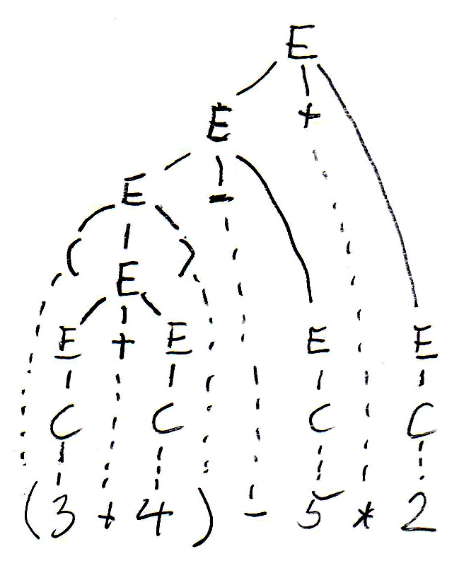
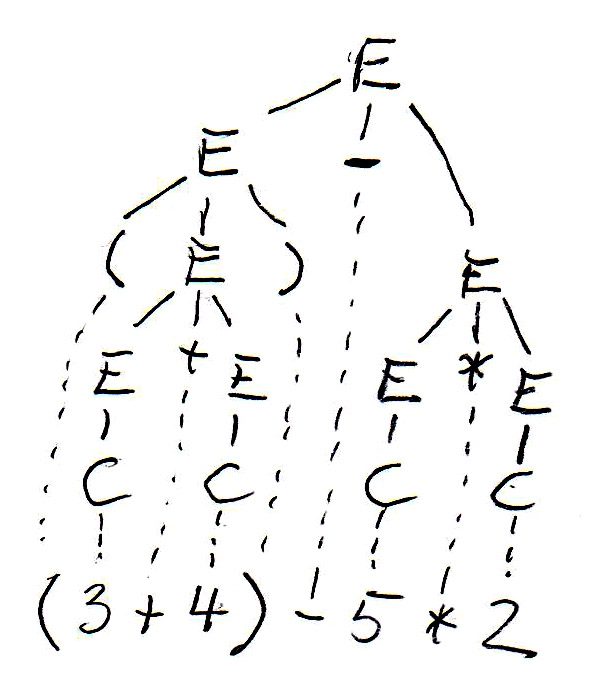
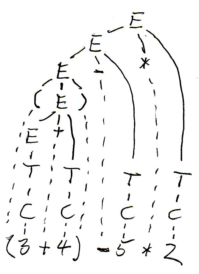
For the expression " (3 + 4) - 5 * 2 ", this grammar gives rise to two different syntax trees as follows:
|
|
The syntax tree guides the evaluation of the expression (which is the meaning of an expression - we want to know what the value of the expression is). Subexpressions within parenthesis must be evaluated first - this gives rise to bottom-up evaluation over the syntax tree.
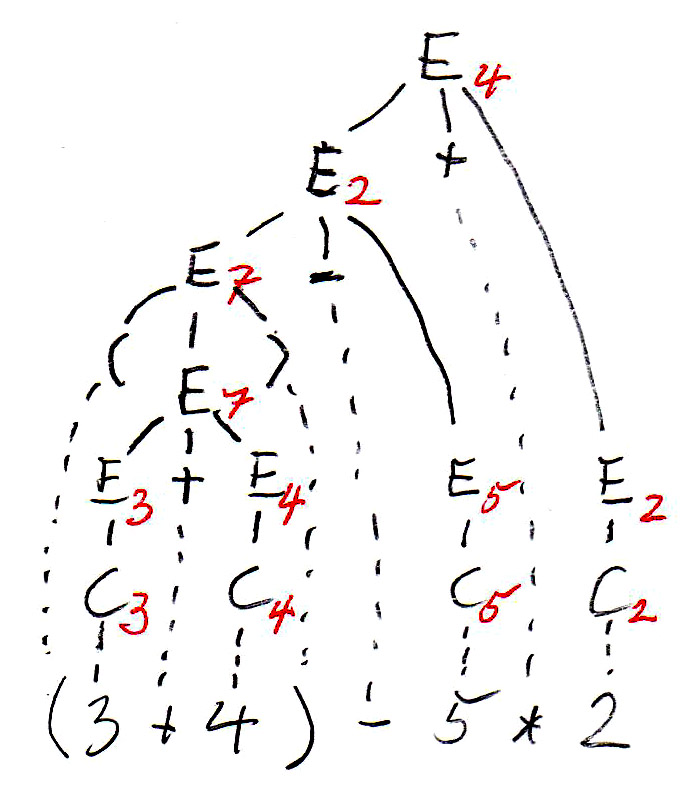
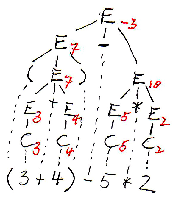
In the syntax trees are copied below, and the non-terminal symbols of the tree (which represent subexpressions) are annotated with their values. We see that the two trees define different values for the same expression. This is because the left tree corresponds to left-to-right evaluation (which is the common way of evaluating expressions), while the right tree corresponds to right-to-left evaluation. We see that this grammar is ambiguous since it gives rise to two different meanings (semantics) for the same expression (sentence). In order to avoid this problem, we have to find an equivalent grammar for expressions that is not ambiguous.
 |
 |
Equivalence: Two grammars are equivalent if they generate the same language. (Already seen earlier)
Ambiguous sentence: A sentence is ambiguous if the syntax rules allow the construction of two different syntax tree for the given sentence.
Ambiguous grammar: A context-free grammar is ambiguous if there exists a sentence accepted by the syntax that is ambiguous.
Coming back to our example, the following Grammar-E2 is unambiguous and equivalent to Grammar-E1:
For the expression " (3 + 4) - 5 * 2 ", this grammar gives rise to the following syntax tree (on the left side):
 |
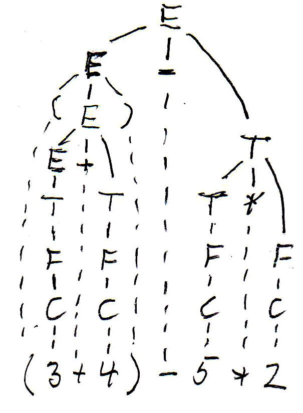 |
As you can see, Grammar-E2 defines left-to-right evaluation for expressions, but does not give priority to multiplication over + and -. Since we always have bottom-up evaluation for expressions, we can introduce another nonterminal F, called "factor", which will always be below the nonterminal T, called "term", in the syntax tree (and therefore evaluated first), if we define Grammar-E3 as follows:
Now we get the syntax tree for the expression " (3 + 4) - 5 * 2 " shown above (on the right side).
Considering programs as strings of characters (or strings of lexical tokens) is fine for deciding whether a given string is a valid program, but it does not tell us what the meaning of the program is. In order to talk about the meaning of a program or of a spoken sentence, it is normally necessary to analyse the different parts of the program (or sentence) and find the meaning of the different components and their inter-relationships. One usually identifies different classes of components and identifies their relationships. Each class normally represents a concept (or construction) of the language. Therefore, one sometimes uses UML class diagrams to represent these issues. Such a class diagram is often called a meta-model or abstract syntax of the language.
These concepts are quite intuitive. Here is an example from the Java programming language to explain the issues. We consider only a small subset of the Java semantics, namely Java statements (assignment, if and while statements) that use variables and expressions. Here is a UML Class diagram showing the relationship between these concepts.
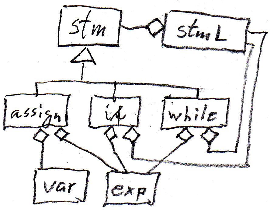
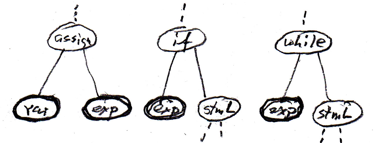
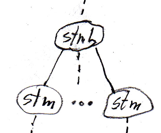
We can represent the "contains" relationships in the diagram by syntax rules as shown in the following table (assign is an assignment statement, if is an if-statement without else, while is a while-statement, stm is a statement, and stmL is a list of statements). Note that these abstract syntax rules are less abstract than the meta-model, since they introduce an order from left to write for the dependent components of an entity.
|
  |
The inheritance relations may also be represented by syntax rules (in the sense of "can be defined as") as follows:
Note that in this context (where we ignore the details of the variables and expressions) the concepts var and exp can be considered as terminal symbols; the other symbols are non-terminals.
Let us consider the Java statement
if (b) {while (a < 10.0) {a = a + addOn();} supplement = a - 10.0;}
Using the above abstract syntax rules and considering var and exp as terminals, then the above Java statement corrresponds to the following sequence of terminal symbols: " exp exp var exp var exp " . This string, by itself, is not very interesting.
However, if we interpret the above abstract syntax rules as rules for constructing a syntax tree, we get a much more interesting result. Each syntax rule defines a possible relationship within the syntax tree, as defined by the tree fragments shown in the table above. We get the following tree for the example Java program, which clearly shows the structure of the program example - which is important for the understanding of the meaning of this program.
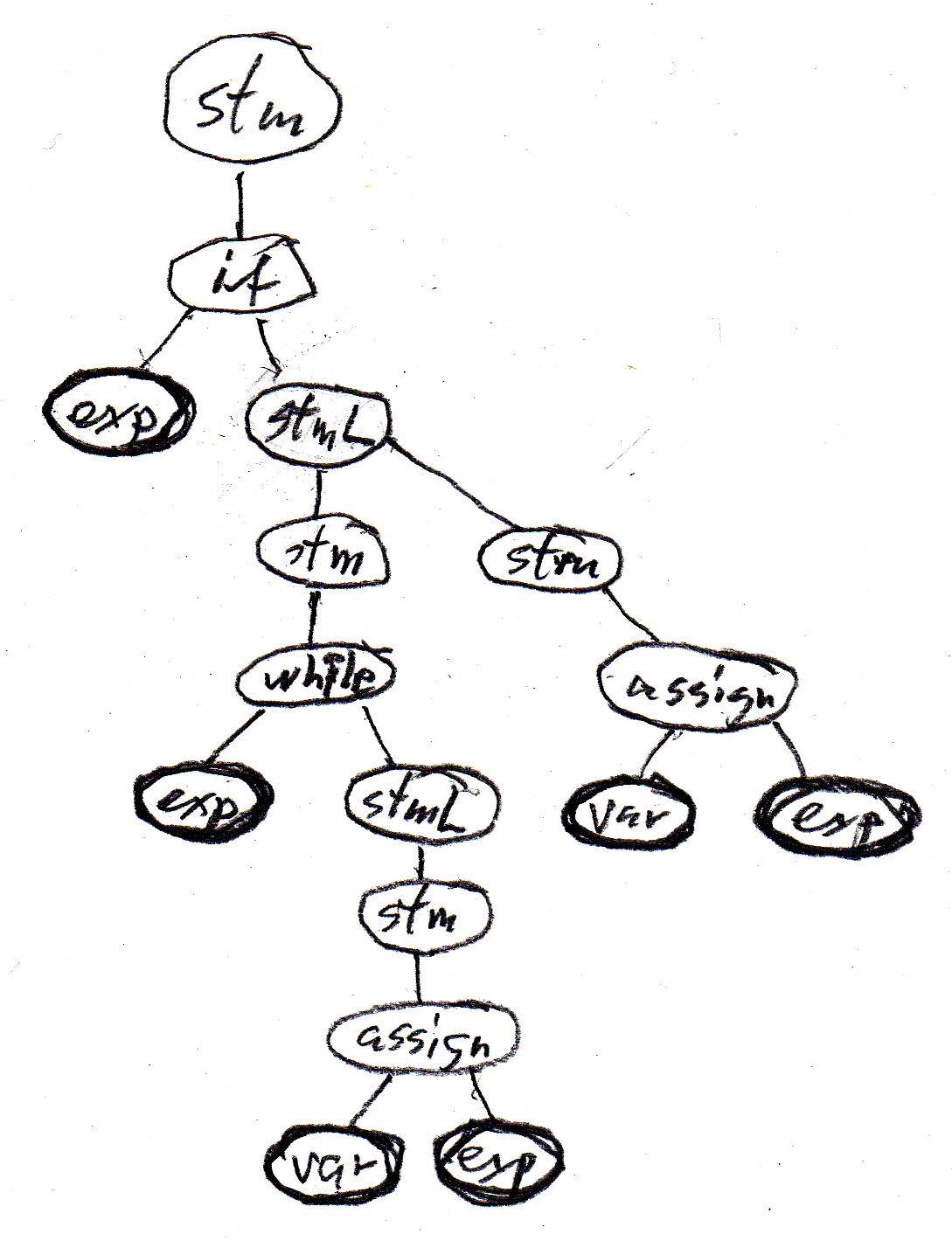
Note that all possible syntax trees can be constructed by interative substitution from the syntax (or syntax tree) rules.
In order to reduce the number of synax rules, one often sees grammars where the inheritance relationships are not explicitly shown. For instance, the seven rules of our example above could be replace by the following four rules, which form an equivalent grammar. Note, however, that in this case the rules for if and while statements are identical (which means that the abstract syntax cannot distinguish them) - this difficulty disappears when "syntactic sugar" is added (see below).
The abstract syntax tree is good for understanding the meaning of a program, but not good enough to analyse a given program given in the form of a string of symbols. For instance, if we change (in the example program above) the if-statement to a while-statement, the sequence of resulting terminal symbols is also " exp exp var exp var exp " - this means we cannot distinguish these two programs by their sequence of abstract var and exp instances. Also a program of the form " if (b) {while (a < 10.0) {a = a + addOn(); supplement = a - 10.0;}} " would have the same sequence of abstract terminal symbols, although the structure of its abstract syntax tree is clearly quite different.
As we have seen above, the abstract syntax for the Java statements is ambiguous. In order to avoid such difficulties, one normally defines a so-called concrete syntax which complements the abstract syntax (the meaning) by introducing additional lexical elements that must be included in the program text, and which are selected in such a manner that any ambiguity is avoided.
For instance, the left concrete syntax below corresponds to what the designers of Java have decided about the syntax of statements. The syntax on the right corresponds to the Pascal programming language. Both have the same abstract syntax and meta-model - and the same meaning for their statements - only the "syntactic sugar" is different. The "syntactic sugar" is written in red.
|
|
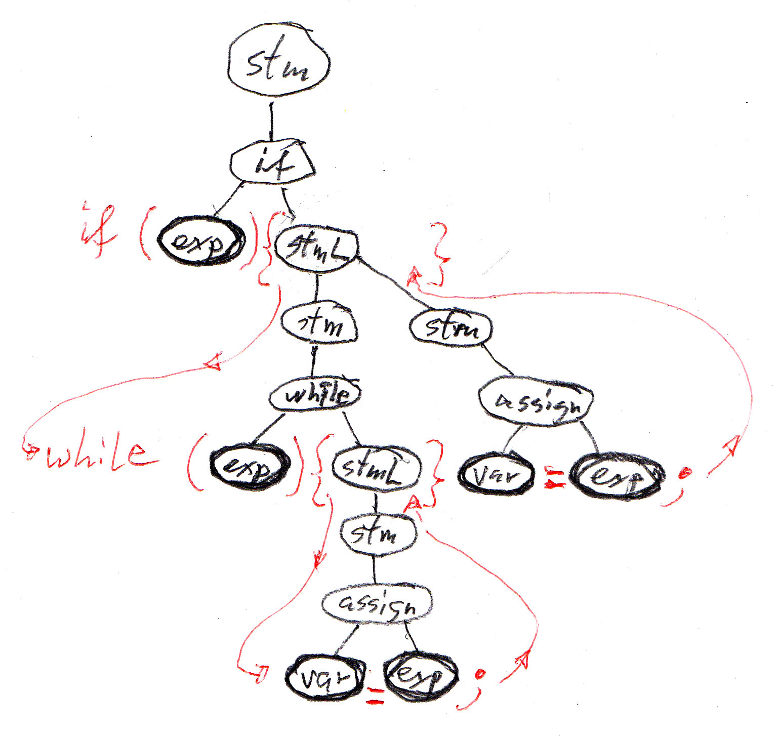
With the Java concrete syntax given above, the abstract syntax tree of the example program becomes the syntax tree of the program shown below, which has a sequence of terminal symbols that correspond directly to the token sequence of the program text.
XML defines a character string representation of abstract trees, called DOM ("document object model"), which is often used for representing objects when they are transmitted over a network or stored as a character string in a database. In XML, each node of the abstract tree is called an "element", and elements may be of different types. The string representation of these elements and their subtrees follow a standard encoding convention that uses the names of the element types in the string encoding. Each element type may have attributes, and all elements have a kind of default attribute which is a character string.
The abstract syntax tree of the Java program above, when encoded as an XML string, may look as follows (note that the indentation has no meaning, it is only introduced to make the string more readable). In this case, all elements have no attributes, nor any default attribute string. The tokens <xxx> and </xxx> represent the beginning and the ending of an element of type "xxx" and its subtree. A token <xxx/> represents a "terminal" element without any subtree.
or (without indentation): <if> <exp/> <stmL> <while> <exp/> <stmL> <assign> <var/> <exp/> </assign> </stmL> </while> <assign> <var/> <exp/> </assign> </stmL </if>
Here are two grammars that define the language defined by the regular expression c c* (a | b).
|
Grammar G1
|
Grammar G2
|
If one uses the grammar G2 to analyze the sentence "c c c a", one may construct the syntax tree by considering the following sequence of intermediate "sentential forms". At each step, one nonterminal in the current sentential form is replaced by the right side of one of the alternative syntax rules for this nonterminal. In the following, each line is a sentential form, and the nonterminal replaced in the next sentential form is shown in blue.
S
Such a sequence is called a "derivation". One may also consider derivations more systematically, for instance, left-most derivations (where always the left-most nonterminal is expanded) or right-most derivations. The following is a right-most derivation for the same sentence using grammar G1:
S
And here is a left-most derivation for the same sentence using grammar G2:
S : there is only one rule for S; it leads to
In the last derivation, in order to decide which rule to apply for the next step, it was sufficient to look at the non-terminal one position to the right to the prefix of the sentence that was already included in the (partially constructed) tree (shown in green). One calls this "look-ahead" of one symbol. The analysis was done by constructing the tree from the top down; this is called top-down analysis. For any grammar in general, one can not always work with a bounded look-ahead. For example, if we use the grammar G1 for top-down analysis, we have to decide at the beginning which of the two rules for S should be applied; however, in order to make this decision, one has to look ahead up to the last symbol of the sentence (which could be a or b). Since the sentences have no bounded length, there is no bounded look-ahead of k symbols (for any given k) that is sufficient to make such a decision for all sentences. Top-down syntax analysis with a k-symbol look-ahead is called LL(k) analysis (first L for "from left to right" and second L for "left-most derivation").
Another popular analysis technique is LR(k) (which stands for "from left to right" and "right-most derivations"). Grammar G1 is suitable for this technique. The syntax tree is built from the bottom up; for instance, consider the right-most derivation with grammar G1 above, starting with the bottom line. At each step, only one next symbol from the input string needs to be considered to make the decision about what syntax rule to apply; see below, where the next symbol is written in red and the nonterminal (in the next higher line) whose production was applied is written in blue.
S
LL(k) and LR(k) parsing methods are deterministic: at each step, a deterministic decision can be made about which syntax rule to apply to build the syntax tree. This implies that the grammar must be non-ambiguous, since an ambiguous grammars may allow for several syntax tree for a given input string. However, there are also non-ambiguous grammars that do not allow for LL(k) nor LR(k) parsing.
It is important to note that one can always (for any context-free grammar) do bottom-up or top-down analysis if one allows for a non-deterministic approach (similar to non-deterministic automata). However, such a procedure is in general not very efficient - because of the need for backing up in case of an unsuitable choice of production rule. Therefore one is interested in grammars that allow deterministic parsing. If a grammar allows for deterministic top-down [or bottom-up] analysis with k symbols of look-ahead, one says that the grammar is LL(k) [ or LR(k) ]. For allowing such parsing methods, the grammars must satisfy certain conditions (which will be discussed below for LL(1) grammars).
Note: In contrast to non-deterministic automata, in the case of context-free grammars that do not allow deterministic LL(k) nor LR(k) parsing, there is no algorithm to find an equivalent grammar that allows deterministic parsing. We saw that this is different for regular languages: for a non-deterministic accepting automaton, there is an algorithm for finding an equivalent deterministic one.
Here is another example of a grammar: Grammar G3:
Here is a left-most derivation of the sentence "a b e d c $" (where $ repesents the end of the string - end of file). In each line, the left-most nonterminal, which is replaced in the next line by the right side of one of the syntax rules, is written in red. The replacement is written in italic. On the right is the corresponding syntax tree (terminal symbols underlined).
Left-most derivation
|
Look-ahead input symbol
|
Syntax tree |
In order to perform a deterministic top-down syntax analysis with a single symbol of look-ahead, we have to decide for each line of the derivation, which syntax rule is to be applied for the left-most nonterminal (written in red), based solely on the information provided by the next input symbol, which is a symbol of the given sentence (line 10) which is written in the position below the nonterminal in question (the next terminal symbol which is not yet part of the syntax tree at this point of the derivation). This means the choice of the alternative (if there is more than one alternative) depends only on the left-most nonterminal and the next input symbol.
It is therefore natural to construct a so-called parsing (or syntax) table that indicates for each nonterminal of the grammar and each input symbol which syntax rule (i.e. which right side) should be applied. Note that for certain nonterminals, certain input symbols should not be the next one - if they are, this represents a syntax error of the input string. Here is the parsing table for the grammar G3 (en empty table entry represents a syntax error). Note: A bnlack entry in the table is the right side for which the symbol of the column is in the First; a blue entry indicates that the symbol of the column is in the Follow of the nonterminal of the table row (and the entry is the right side which could generate the empty string).
| a | b | c | d | e | f | $ | |
| S | A B C | A B C | A B C | A B C | A B C | ||
| A | D B | C | C | C | C | D B | |
| B | b A d | c | |||||
| C | ε | ε | ε | e C | ε | ||
| D | a | f S |
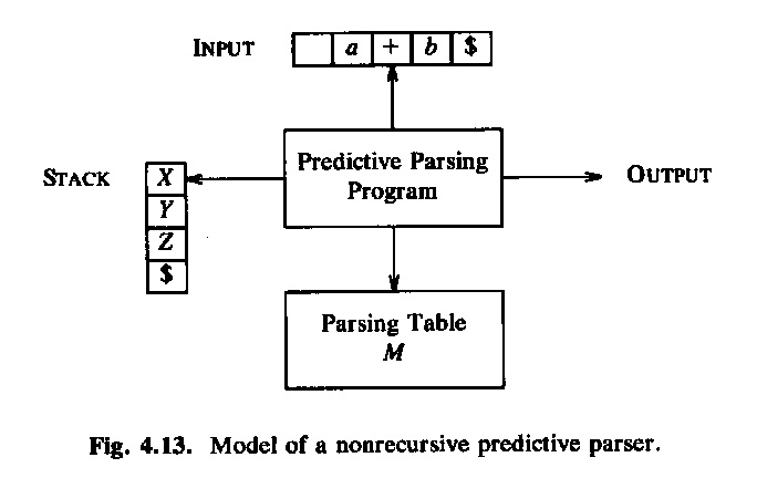
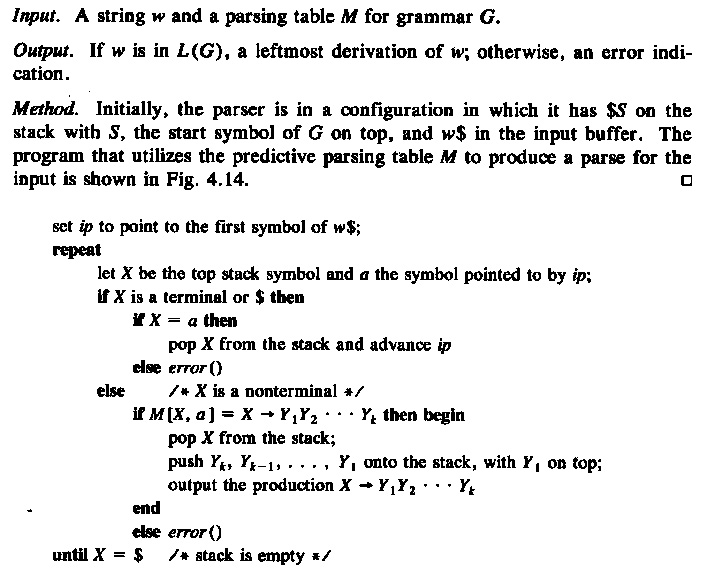
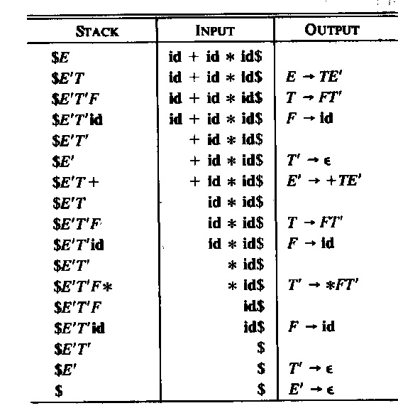
A simple approach to the implementation of LL(1) parsing is to build an interpreter program that uses the information in the parsing table and produces the left-most derivation discussed above. One need a "reading head" that reads the given input string from left to right and always indicates the next symbol to be considered. The other information that the interpreter must remember is the intermediate sentenial form (i.e. the content of the current line in the derivation discussed above). This sentenial form consists of two parts: on the left is the part of the input string that is already included in the partically constructed syntax tree, and on the right is a string of nonterminals and terminals which starts with the left-most nonterminal to be replaced. It is convenient to store this right part in a stack data structure with the left-most nonterminal on the top of the stack. This is the approach used in the interpretive algorithm described in the book by Aho et al. (see below).
Another approach to the implementation of LL(1) parsing is to use recursive procedures, one for each non-terminal of the language. These procedures call one another recursively. Each procedure realizes the rules that are defined for the non-terminal in question. For example, for grammar G3, one could write the following Java procedure (note that the variable char symb contains always the next symbol (the look-ahead) and the procedure next() is used to read the next symbol). The main calls the procedure S() and verifies, when S returns, that the next symbol is end-of-file. Note that the abbreviation "symb in {'a', 'b', 'c', 'e', 'f'}" does not follow the Java syntax and must be rewritten in order to obtain a valid Java program.
|
|
Here is the grammar G3 again:
Please note that each of the following modifications of the grammar G3 will make it non-LL(1):
To avoid problems like under point (1) above, one has to verify for each nonterminal that has several alternatives, that there is no symbol that could be the first symbol of a string generated by one alternatives and also be generated as the first symbol of another string by another alternative. One calls the set of terminal symbols that may appear as the first symbol of a string generated by a nonterminal X, the set First(X). Similarly, one calls First(right side) the set of terminals that could appear as the first symbol of a string generated by the given right side of a syntax rule. To avoid the problems such as under point (1) above, we therefore have the following constraint on the grammar: If a nonterminal has several alternatives, then the First sets of all alternatives must be disjoint (that is, they should not contain any common symbol).
To avoid problems like under point (2) above, we have to check some additional rule if one of the nonterminals may generate the empty string - because in this case the next symbol of the look-ahead may not correspond to the First of this nonterminal, but rather to one of the symbols that may follow the substring generated by the nonterminal within the overall input string. The set of terminals that may follow a string generated by a nonterminal X within the context of a valid sentence of the grammar is called Follow(X). To avoid the problems such as under point (2) above, we therefore have the following constraint on the grammar: If a nonterminal X can generate the emtpy word, then Follow(X) must be disjoint from the First of all alternatives. But this is equivalent to requiring that: If a nonterminal X can generate the emtpy word, then Follow(X) must be disjoint from the First(X). In order to determine whether a nonterminal can generate the empty string, one normally includes the symbol "ε" in the set First(X) if X can generate the empty string (although this symbol is not formally an input symbol).
LL(1) condition: In summary, one can say that a grammar has the LL(1) property if the following two conditions are satisfied by all non-terminals of the grammar:
For all non-terminals, the First sets for all alternative right sides are disjoint.
Note: The rules to calculate the sets First and Follow are formulated in a form which corresponds to the iterative substitution which we discussed at the beginning of this chapter.
The following calculation rules must be applied interatively until there are no further additions to the sets First and Follow. Initially, one may assume that these sets are all empty. The sets First can be calculated first, since they do not depend on the Follow sets. Here is an alternate presentation of this topic.
Example: Calculating the First and Follow sets for the grammar G3
Here is the grammar again
|
Calculating the First sets, starting with the simple cases:
|
Calculating the Follow sets for the nonterminals that can generate the empty string:
Once the sets First and Follow have been calculated, one can check that the grammar is LL(1) by verifying the two properties discussed above. These properties ensure that the parsing table admits at most one alternative in each entry of the table.
In fact, the sets First and Follow are very useful to define the parsing table. We can follow the following procedure to fill in the entries in the parsing table. For an entry for nonterminal X and next terminal symbol y, the entry is found as follows:
(1) Combine common prefixes: If several production rules for the same non-terminal contain some common prefix (for instance A --> a B c | a B A ), one can incorporate this prefix in a new rule (the example becomes A --> a B A' and A' --> c | A ).
(2) Elimination of left recursion: A grammar with left recursion (for instance A --> A c b | a ) leads to infinite loops during the analysis (by recursive procedures, or by using a parsing table). Such a grammar is not LL(1), by the way.
Definition: A grammar has left recursion if it contains a non-terminal, say A, from which it is possible to derive a string " A Y " where Y is any string of terminal and/or non-terminal symbols.
When discussing the alternative definition of Kleene's operator at the beginning of this chapter, we saw that "immediate" left recursion (that is, without any intermediary non-termianl symbol) can be replace by right recursion. This general rule discussed with Example 4 leads to the following elimination recipee:
For more complex cases, one can use the following algorithm (taken from the book by Aho):
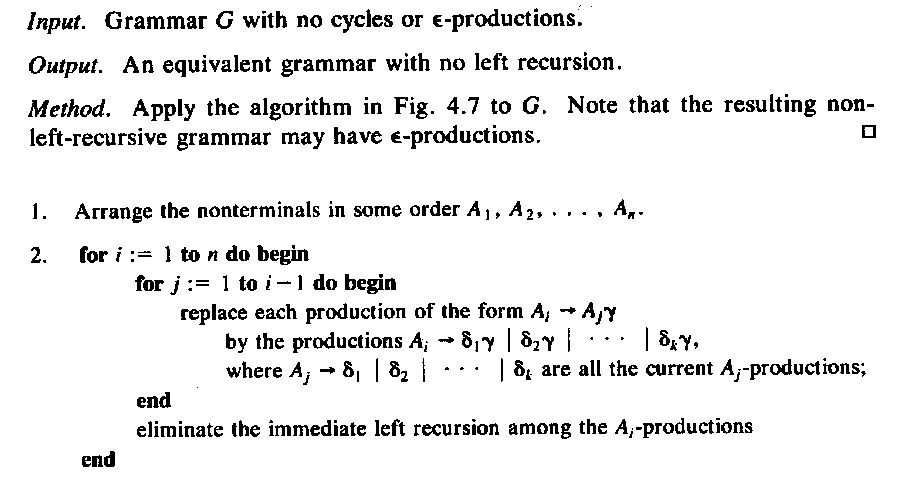
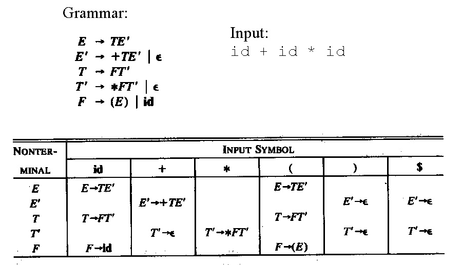
Here is an example grammar for numerical expressions:
Sometimes one uses extended BNF notation for defining the syntax, where parenthesis, Kleene's star and the ?(optional) operator are allowed. Then the right side of a syntax rule could in general define a regular expression involving terminal symbols, but also nonterminals. For instance, we know that the recursive equation " T' = "*" F T' | ε " has the solution T' = ( "*" F )* - notice that "*" is a terminal symbol and the * after the closing parenthesis is Kleene's star operator. Therefore the rules (3) and (4) above could be equivalently rewritten as
Syntactic rules can also be defined in graphical notation similar to state machines. Such syntax descriptions are called "syntax diagrams". Below (left) are such diagrams for the syntax rules (1), (2) and (5). In the middle is a syntax diagram corresponding to rule (6) above. It is important to realize that each syntax graph is a recursive state machine, this means, it behaves like a state machine, except that certain transitions do not correspond to the reading of an input symbol, but instead represent the (recursive) call of another state machine instance. A recursive state machine equivalent to the syntax diagram for T (in the middle) is shown on the right - the double arrow transitions represent the calling of an instance of the F-stateMachine.
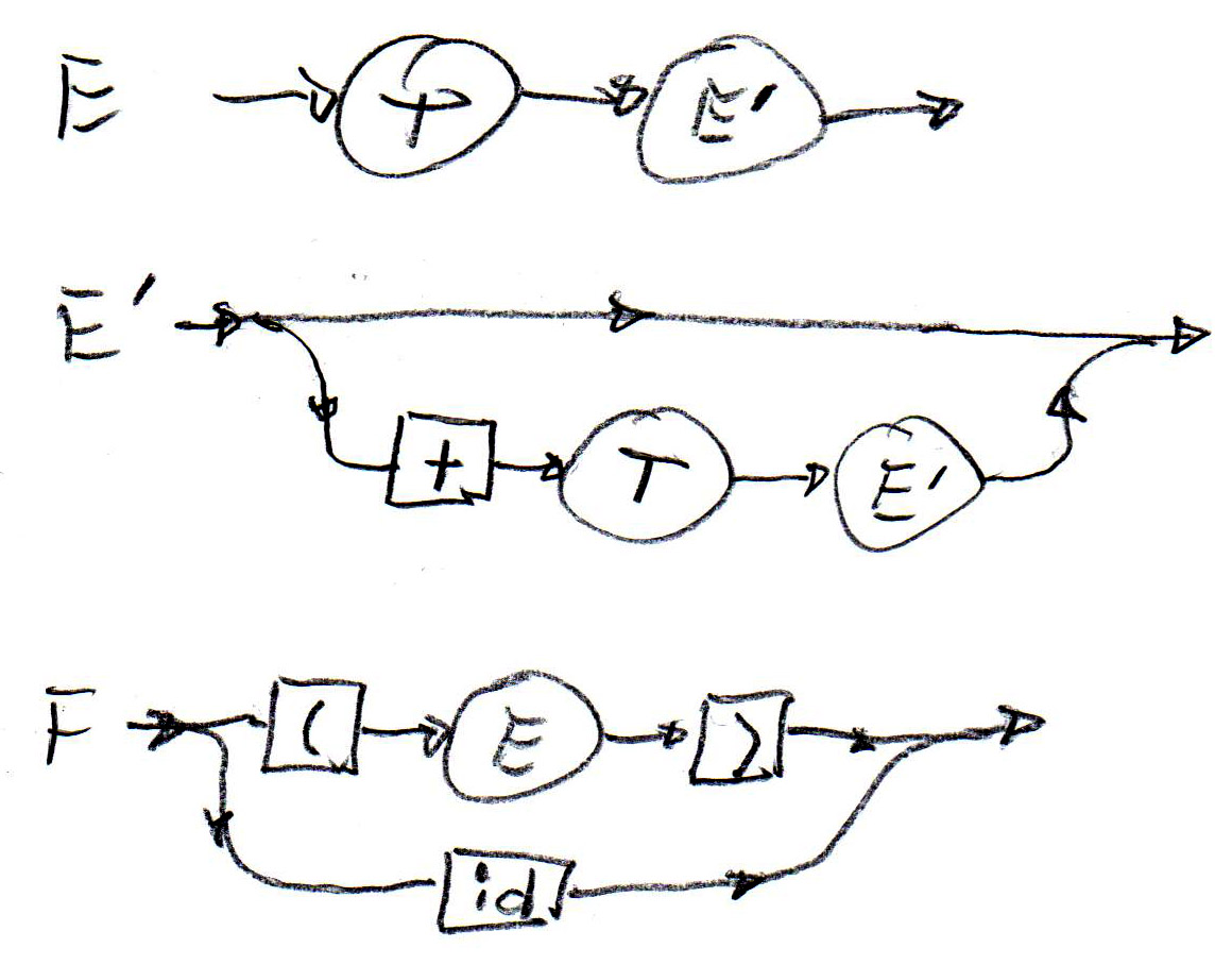 |
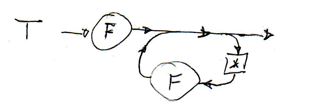 |
Recursive automaton for T:
|
Note that these syntax diagrams (or the corresponding recursive state machines) can be easily implemented by recursive procedures, as proposed for the implementation of LL(1) parsing with recursive procedures. For instance, syntax structures as shown for T above can be easily realized by a method with a loop, such as the following:
When one builds a syntax analyser using recursive procedures, one often tries to reduce the number of procedures as compared with the number of nonterminals in the original syntax. Replacing the rules (3) and (4) by rule (6) and then using the diagram above is an example for such a reduction.
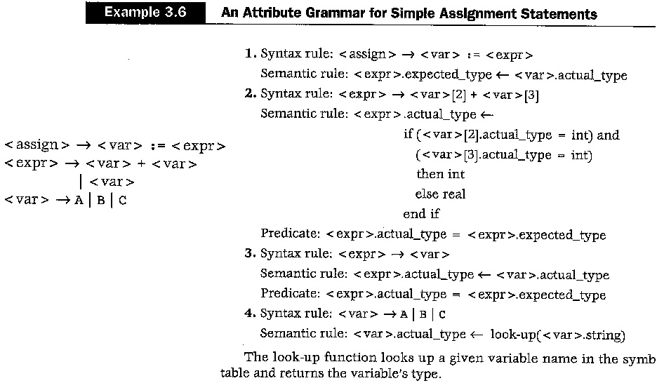
For the description of semantic properties of the syntactic constructs of a language, one often uses so-called semantic attributes - attributes of the syntactic non-terminals (and sometimes terminals). As an example, one may think about the classes of non-terminals defined above in the section on abstract syntax. An expression object may have an attribute defining the data type of the expression, a variable object may have an attribute defining the type of the variable, and a statement and expression object may have an attribute that contains the generated code for representing this object in the generated object code.
See Section 3.5 in the book by Sebesta for an explanation of
the use of semantic attributes, in general,
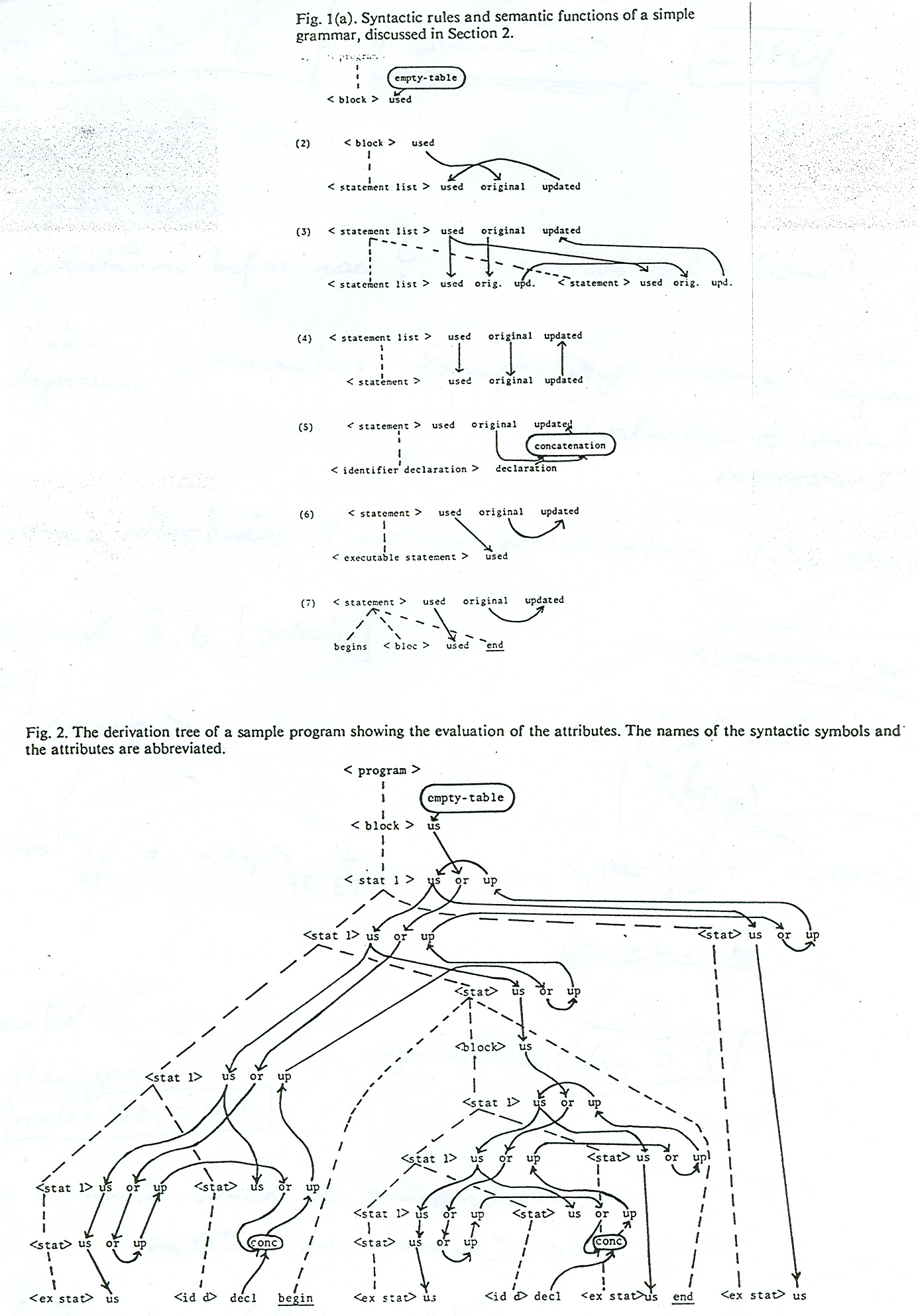
Here are the diagrams showing an example in the book: definition of the attribute grammar, definition + tree example
Note: The attribute evaluation rules, in their restricted form to avoid circular definitions (as mentioned in Section 3.5.3 in the book by Sebesta), were first proposed in my publication "Semantic evaluation from left to right" which appeared in the (then) prestigious journal of the ACM in 1976. Here is an example from that article which shows the rules defining the scoping rules of a programming language; in fact, it shows how the information included in the partial symbol tables is passed between the different parts of the program.
Static evaluation means evaluation during the compilation phase (as opposed to during the execution phase). The evaluation of semantic attributes is performed during the compilation phase. What kind of attributes are required for the evaluation of the value of expressions ? - This depends on the grammar rules. In the following, we want to evaluate the semantic attributes during a single depth-first pass through the syntax tree - that is, in parallel with the syntax analysis using the recursive decent LL(1) parsing approach.
We have seen the following three forms of sytax definition for simple expressions:
E(0) --> T | E(1) + T | E(1) - T
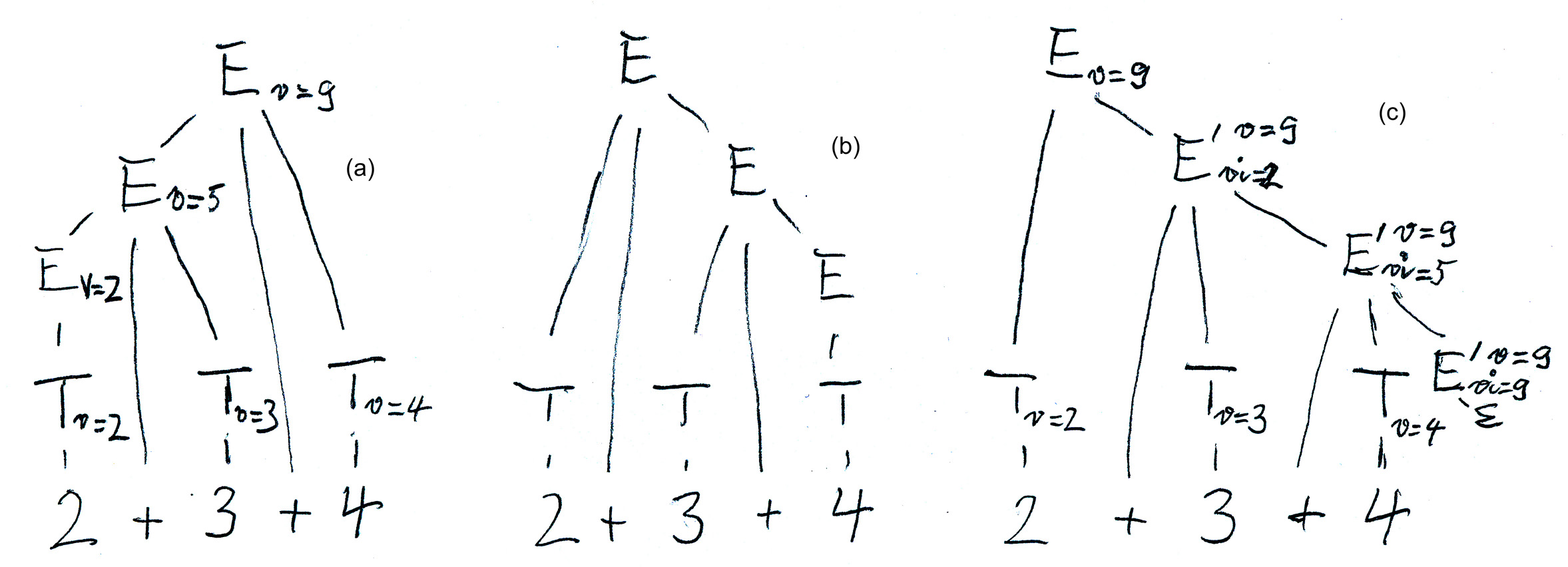
With the grammar (1) we need one synthesized attribute "v" (for value) for the nonterminal E which is evaluated on the syntax tree from the bottom up and from the left to right, as seen in Figure (a) below. - However, grammar (1) is not suitable for LL(1) syntax analysis. - Here are the evaluation rules for the attributes:
for the first alternative: v(E(0) ) := v(T)
With grammar (3), which is obtained from grammar (1) by applying the transformation rule discussed earlier, we get a syntax tree as shown in Figure (b) below. With bottom-up attribute evaluation, we get an evaluation from the right to the left, which is not what we need. However, we can introduce two attributes for E', a synthesized attribute called "v" (as for the nonterminal E above), plus an inherited attributed called "vi" which represents the intermediate value of the expression evaluated up to the non-terminal node E' in question. Here are the evaluation rules for the attributes (see also Figure (c) below):
for the rule E --> T E' : vi(E') := v(T) --- v(E) := v(E')
Here is a sketch of a recursive procedure realizing the syntax analysis and semantic evaluation for E'. Note that the synthesized attribute is simply programmed as a value returned by the parsing procedure, and the inherited attribute is simply represented by a parameter of the procedure.
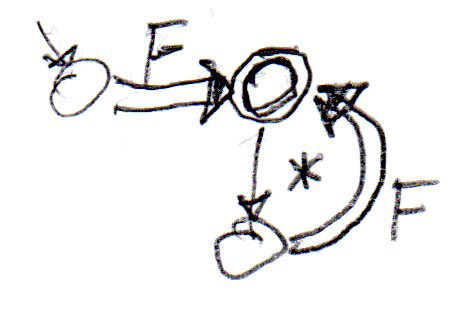
With grammar (2): We note that the attribute evaluation rules for grammar (3) are complicated. The situation becomes much simpler if one uses the grammar (2). It also has the advantage over grammar (3) that it has only one nonterminal, and therefore a single recursive procedure is enough (instead of two, one for E and one for E' in the case of grammar (3)). The following is a sketch of such a recursive procedure written in Java according to the syntactic diagram below.
![]()
Chomsky distinguished the following four classes of grammars (from the most general to the most restrictive form):
General grammar: The grammar is a set of production rules, where the left side and the right side of each rule are strings of non-terminal and terminal symbols. A rule "left side" --> "right side" means that the string "left side" can be replaced within a derivation by the string "right side".
A (formal) language is a subset of all the symbol sequences that can be formed from the alphabet of the terminal symbols. In general, there is no bound on the length of these sequences (the sentences of the language), most languages are infinite (that is, have an infinite set of sentences). Therefore the following questions arise:
How can we define such an infinite language using a finite description ? - One needs a finite description to reason about it.
A problem is undecidable if it can be shown that there exist no algorithm that makes a decision for all possible cases. - In a sense, one may say that the problem is "more complex" than problems that are NP complete, because for those problems there are algorithms, although not very efficient.
Examples of undecidable problems:
Halting problem of Turing Machines (this is a very famous example, because in this context, the existance of undecidable problems was detected by Turing) - here is a simple proof
Note: All questions related to regular languages are decidable.
Translated from French and revised: Februar 2008; updated 2009, 2010, 2011, 2012, 2013, March 16, 2015
.jpg)